Likelihood by direct simulation: Consett measles example

Author

Aaron A. King and Edward L. Ionides

We’re going to demonstrate what happens when we attempt to compute the likelihood for the Consett measles outbreak data by direct simulation from the full latent state distribution.

First, let’s reconstruct the toy SIR model we were working with.

source("model_measSIR.R")

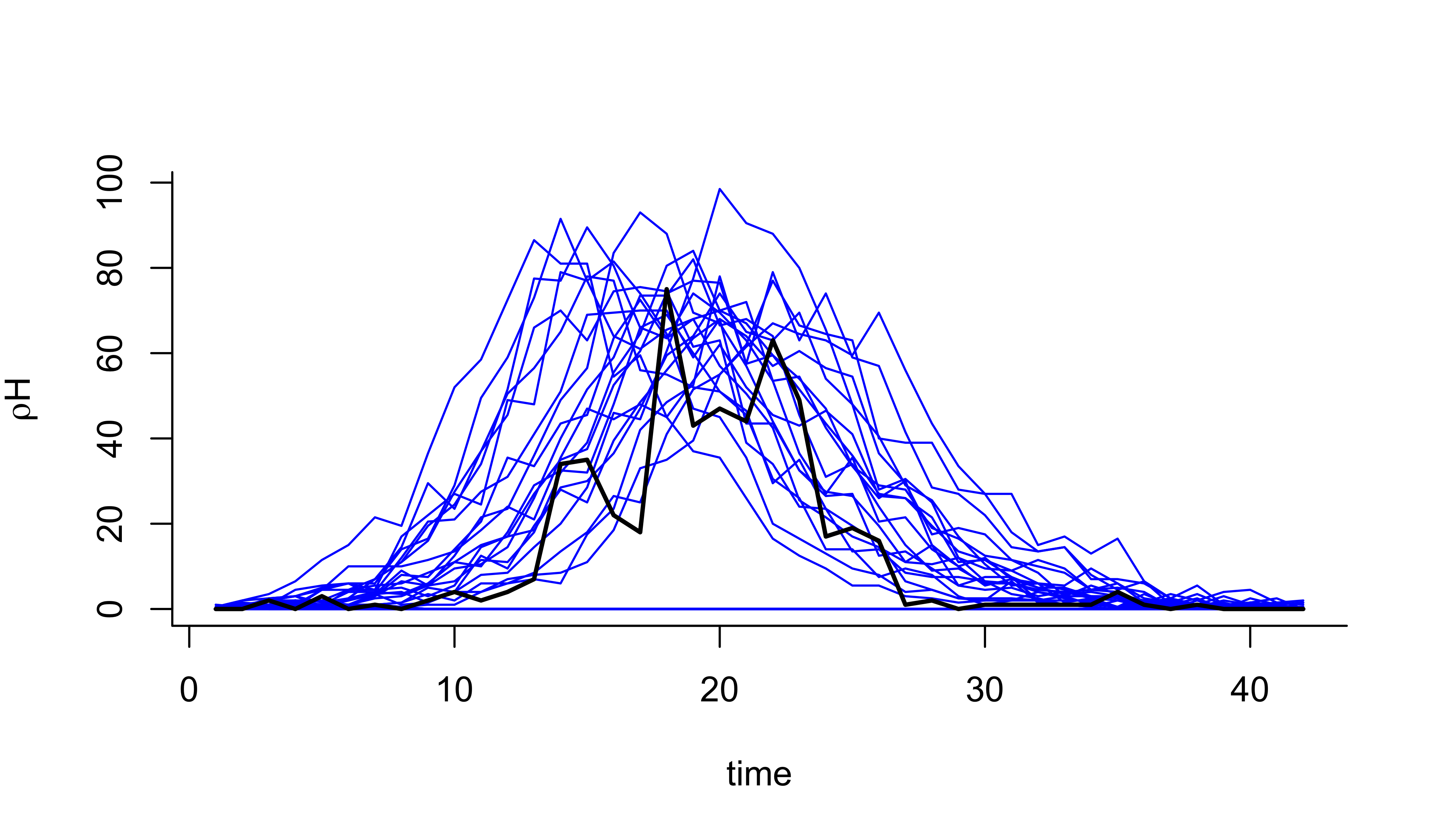
Let’s generate a large number of simulated trajectories at some particular point in parameter space.

measSIR |>
  simulate(nsim=5000,format="arrays") -> x
measSIR |>
  emeasure(x=x$states) -> sims
matplot(time(measSIR),t(sims[1,1:50,]),type='l',lty=1,
  xlab="time",ylab=expression(rho*H),bty='l',col='blue')
lines(time(measSIR),obs(measSIR,"reports"),lwd=2,col='black')

We can use the function dmeasure to evaluate the log likelihood of the data given the states, the model, and the parameters:

ell <- dmeasure(measSIR,y=obs(measSIR),x=x$states,times=time(measSIR),log=TRUE,
  params=coef(measSIR))
dim(ell)

[1] 5000   42

According to the general equation for likelihood by direct simulation, we should sum up the log likelihoods across time:

ell <- apply(ell,1,sum)
summary(ell)

   Min. 1st Qu.  Median    Mean 3rd Qu.    Max. 
   -Inf    -Inf    -Inf    -Inf    -Inf  -125.1

summary(exp(ell))

     Min.   1st Qu.    Median      Mean   3rd Qu.      Max. 
0.000e+00 0.000e+00 0.000e+00 1.775e-58 0.000e+00 4.901e-55

The variability in the individual likelihoods is high and therefore the likelihood esitmate is imprecise. We will need many simulations to get an estimate of the likelihood sufficiently precise to be of any use in parameter estimation or model selection.
What is the problem?
- Essentially, very few of the trajectories pass anywhere near the data and therefore almost all have extremely bad likelihoods. Moreover, once a trajectory diverges from the data, it almost never comes back. While the calculation is “correct” in that it will converge to the true likelihood as the number of simulations tends to \(\infty\), we waste a lot of effort investigating trajectories of very low likelihood.
- This is a consequence of the fact that we are proposing trajectories in a way that is completely unconditional on the data.
The problem will get much worse with longer data sets.

Produced in R version 4.4.0.